Identifiers

We've learned how to write mathematical numbers and character strings as literals. R also has a few built-in constants. One of them is the number pi, which is the circumference of a circle divided by its diameter, or about 3.1416:

> pi [1] 3.141593 >

Here, pi is an identifier. When we type an identifier into the system, R attempts to evaluate it. In the case of pi, R already has a value bound to pi. The system is able to correctly evaluate pi. Whenever pi is used in an expression, the symbol pi is replaced by the value it is bound to, namely the floating point number which is approximately 3.141593. The expression is then evaluated using this value:

> 2*pi [1] 6.283185 > cos(pi) [1] -1 >

We have already seen identifiers when we have used functions. For example, in the preceeding computation, cos is an identifier. When we type it, the R system evaluates it, yielding the cosine function.

> pi [1] 3.141593 > cos .Primitive("cos") >

In the first line, we typed the identifier pi, and the system evaluated it to yield the familiar value. In the second line, we typed cos, and the system evaluated it. Here, cos is evaluated to yield a representation of the cosine function. Just as pi evaluates to 3.141593, cos evaluates to the cosine function. The system can easily represent a floating point number to us (such as 3.141593), but it displays the function simply as .Primitive("cos").

The symbol pi is bound to some floating point data value, namely 3.141593. The symbol cos is bound to a different kind of data, namely, an R function which computes the cosine.

We have now seen five different kinds of things which can be typed in to R:

•   Numeric literals, such as 4, -10, 3.141593, 3e8, -4e2, or -1e-3.
•   Character literals, such as "CA", "94102", or "\"quoted\"".
•   Boolean literals, such as TRUE
•   Operators, such as +, *, or ^
•   Identifiers, such as cos, sqrt, or pi.

Identifiers in R always consist of letters, digits, and the dot (period) character. But they may not begin with a digit, and they may not begin with a dot followed by a digit. Those coming to R from a Fortran, SAS, or Common Lisp background must remember that case matters in R: Cos is not the same thing as cos:

> Cos(pi) Error: couldn't find function "Cos" >

When you mispell a function name, you will often see this error. Of course, if you mispell cos as sqrt, you will see something different.

Those who are coming to R from C should remember that the underscore character is NOT allowable in an identifier in R. Note: this has changed in recent versions of R.

Assignment

So far we have used identifiers with built-in values. R already knows what pi, sqrt, and cos do. These identifiers are already bound to values.

But we can bind values to our own identifiers by using the assignment operator:

> xx <- 3 >

Here, we bound the value 3 to the symbol xx. Notice that the system did not echo back any value, but returned with the command prompt. But if you then ask the system to evaluate xx, it responds with the correct value:

> xx <- 3 > xx [1] 3

The symbol <- is normally pronounced "gets". At one time, the underscore character _ could be used as a substitute for the gets symbol, and you should keep this in mind if you wind up having to use old S or R code.

Beware the following gotcha. If you are testing whether or not something is less than a negative number, and you run the less than sign together with the minus sign, the result will be interpreted as gets. And you probably did not want that. Here is a simple example where we want to print an error if a number aa is less than -3:

> aa <- 500 > if (aa<-3){print("error")} [1] "error" > aa [1] 3

Notice what happened; everything went wrong. First of all, even though the value of aa started out at 500, we still printed the word "error". Worse, aa got turned into a 3. This is because <- is always parsed as a single token (or single fundamental element of the language). We should have put a single space to separate the < from the -:

> aa <- 500 > if (aa< -3){print("error")} > aa [1] 500

This time, all's right with the world. The "error" message never gets printed (as it shouldn't), and aa's value is unharmed.

Once you have bound a value to an identifier, the identifier may be used in computations. Whenever the identifier is seen, the interpreter tries to evaluate it. If there is a value associated with it, the value is used in place of the identifier:

> xx <- 3 > xx^2 [1] 9

If there is no value associated with the identifier, then an error results:

> xx <- 3 > xy Error: Object "xy" not found

The system is letting you know that there is no value associated with xy. It understands xx, but not xy, because we have not given a value to xy.

The use of identifiers may make a calculation transparent to a human reader:

> baseline.pop <- 117 > n.cases.one.yr <- 12 > py.noncases <- baseline.pop-n.cases.one.yr > py.cases <- n.cases.one.yr/2 > incidence.rate <- n.cases.one.yr/(py.cases+py.noncases) > incidence.rate [1] 0.1081081

When we type an expression such as incidence.rate <- n.cases.one.yr/(py.cases+py.noncases), the expression on the right hand side of the assignment operator <- is first evaluated to yield a result. This result is then bound to the identifier on the left hand side.

An assignment occurs when the flow of control reaches it. Normally, this happens one time, when you enter the assignment statement at the command prompt. Later, we will see that you can have a file of R commands that can be loaded into the system. Statements (or statement blocks, which you will see later) or normally executed in order, one at a time, starting at the top. Notice that once an assignment statement has occurred, the symbol which you bound is available to further statements.

However, if I later change the value associated with an identifier, the changes do not propagate; other values which depended on the value of the identifier I just changed are not affected. Rather, the assignment statements have to be run again:

> baseline.pop <- 117 > n.cases.one.yr <- 12 > py.noncases <- baseline.pop-n.cases.one.yr > py.cases <- n.cases.one.yr/2 > incidence.rate <- n.cases.one.yr/(py.cases+py.noncases) > incidence.rate [1] 0.1081081 > baseline.pop <- 1000 > incidence.rate [1] 0.1081081

R has excellent facilities for encapsulating and repeating complex compuations, which we will see later.

One more note. It is good style to choose identifiers that are meaningful to a human reader. Single letter identifiers such as i and a are particularly evil, since they can be difficult to search for in a program file.

Function Calls in Expressions

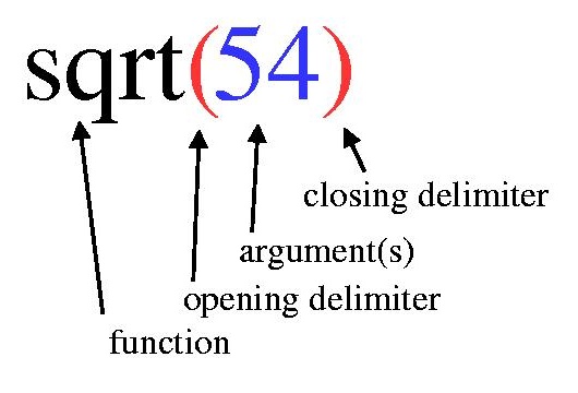
Recall that a function call looks like this:

We can use a variety of values for the argument:

> sqrt(54) [1] 7.348469 > sqrt(2e-6) [1] 0.001414214 >

And we can use a variety of values for the function itself:

> log(54) [1] 3.988984 > is.numeric(54) [1] TRUE > abs(54) [1] 54 >

So the pattern for a function call involves an identifier for the function, then the opening parenthesis, then the argument (or arguments), and the closing parenthesis. And if there is more than one argument, then they must be separated by commas:

> log(1000,10) [1] 3 > log(10,1000) [1] 0.3333333 > sqrt(54,10) Error: 2 arguments passed to "sqrt" which requires 1. >

As we discussed last time, the logarithm function can be called either with one argument (in which case) it calculates the natural logarithm, or it can be called with two arguments, in which case the logarithm of the first number is calculated with the second number as the base. And it matters which number goes in which argument place; log(10,1000) is very different from log(1000,10). But sqrt is not set up to take more than one argument.

In R, you can use an expression that returns a number in a place where a number is expected. So we can do things like this:

> sqrt(50+4) [1] 7.348469 > 50+sqrt(16) [1] 54 > sqrt(50+sqrt(16)) [1] 7.348469 >

What is happening? The function sqrt requires a single argument which must be numeric. But we first entered sqrt(50+4). What happens is the expression 50+4 is evaluated to yield 54, and then the 54 is given to the sqrt function. In the second case, we first take the square root of 16, and then the resulting 4 is added to 50. In the final case, we take the square root of 16, add it to 50, and then take the square root of the whole thing.

As before, we use grouping parentheses to make sure that the components of an expression are evaluated in the order we wish:

> (2+sqrt(2*(3+5)))^3 [1] 216 >

Here, the 3+5 happens first, then the 2*. Then the square root is taken (yielding 4); 2 is added, and finally the resulting 6 is raised to the third power, yielding 216.

Here is another example:

> 4^3^2 [1] 262144 > (4^3)^2 [1] 4096 > 4^(3^2) [1] 262144 >

What this shows is that the power operator ^ is evaluated from right to left when we don't otherwise specify. On the second line, we used grouping parentheses to see to it that 4 is first raised to the third power, and then the result is squared. On the third line, we first square 3 yielding 9, and then raise 4 to the 9th power. The first line without grouping parentheses yields the same result.

In R, we have seen two uses of parentheses: (1) to surround the argument list in a function call, and (2) to group subexpressions to specify the order of operations.

Defining functions

So far, we have always been using literals as the argument of a function. And we've used an identifier of the function we wish to call. We've called several basic built-in functions this way.

It is important to realize that in R, functions themselves are a kind of data, just like the numeric, character (text, string), and boolean data we've seen. And just as there are numeric literals, character literals, and boolean literals, there are expressions which are in some ways may be considered as function literals.

Let's consider a function to square its argument. We could square any number by simply using the caret:

> 54^2 [1] 2916 >

But this is fine for one number, or a few numbers. But to write a function to do this, we use the following:

> function(x){x^2} function(x){x^2} >

The format for a function definition begins with the word function. After this, we have an open parenthesis, followed by an identifier (in this case, x), and finally a close parenthesis. We then have an expression in curly braces¹. The identifier in the parentheses is a local name for whatever the argument of the function is. In the expression between the braces, we do whatever computation we mean to do with the argument of the function. Here, we square the argument by writing ^2 after the identifier, just as we square a constant.

Inside the example square function, the argument is called x. Every time we call the function with a different argument, the symbol x has a different meaning. If we call the function with argument 54, then x will be evaluated as 54 inside the function, until the call is over. If we call the function with argument 1e-3, then x will be evaluated as 1e-3 inside the function, until the call is over. And once the function call is over, the value of x is forgotten.

So let's try it:

> (function(x){x^2})(54) [1] 2916 >

Notice that (function(x){x^2}) takes the same place that sqrt or log did. The form of the function call is exactly the same as before: we have the function, followed by the opening parenthesis, the argument(s), and the closing parenthesis. The green parentheses are the same function call parentheses you've seen all along.

But before we were using built in library functions like sqrt, and we typed sqrt(54). But here, we use our own function (function(x){x^2}) instead of an identifier for a library function. Note that our function must be enclosed in grouping parentheses so that R knows where the function definition ends.

When we used our function to square 54, the symbol x was bound to the value 54, so that whereever an x appears, it is replaced by the numeric value 54. So the expression x^2 is treated as 54^2. R evaluates 54^2 to yield 2916.

> (function(x){x^2})(54) [1] 2916 > (function(x){x^2})(3) [1] 9 >

What just happened? We first used the function to square 54 as before; the argument was the numeric literal 54. Then we called the function again, with 3 as the argument. When the second call happens, the value of x inside the function is replaced by 3. Then the expression x^2 is interpreted as 3^2, and this yields 9. The value 9 is then returned automatically by the function. The previous call had x as 54, but this is all forgotten. It's a new world each time. And the value of x has no meaning on the outside of the function.

Let's do another example. Suppose that I wish to compute the logit of some proportions. The logit transformation is the logarithm of the odds. Recall from basic epidemiology that if p is the probability of some event, then the odds of the event are defined to be p/(1-p). The logit is then the logarithm of the odds. When we compute the logarithm of p/(1-p) from p, we have calculated the logit of p. The logit transform is used frequently in epidemiology and biostatistics as many of you know.

Question. What is the logit if p equals 1? What is the logit if p equals 0? Does it make sense to compute the logit of a number less than zero in epidemiology? Does it make sense to compute the logit of a number greater than 1 in epidemiology?

Let's write a function to compute the logit transform of some numeric proportions or probabilities.

> (function(x){log(x/(1-x))})(0.5) [1] 0 > (function(x){log(x/(1-x))})(0.8) [1] 1.386294 > (function(x){log(x/(1-x))})(0.2) [1] -1.386294 > (function(x){log(x/(1-x))})(0.9) [1] 2.197225 >

This is already useful, since we can keep using the UP keyboard arrow, and changing the number in the argument parentheses (0.5, 0.8, 0.2, 0.9) to different values to recompute the logit. This saves work, and reduces the error chance, since we'd have to change two values if we edited an expression like log(0.8/(1-0.8)) itself. (Of course, for now we're still using duplication to do the job of repetition.)

Question. Explain the meaning of each of the five sets of parentheses in the logit example.

Question. What happens to the logit as the argument gets closer and closer to 1? Use R to find out. Find out what happens as the argument gets closer and closer to zero.

Question. What do you notice about the logit of 0.2, 0.5, and 0.8? Use R to explore a conjecture about the relationship between the logit of 0.5-A and the logit of 0.5+A for different values of A.

Assigning function values to identifiers

Normally, you would not use a function in this way. Rather, you would bind the function to a symbol so you could call it using a meaningful identifier:

> logit <- function(pp){log(pp/(1-pp))} >logit(0.5) [1] 0

Now, our function logit just behaves like a built-in function. When the interpreter gets the symbol logit, it is evaluated just like any other identifier:

> logit function(pp){log(pp/(1-pp))} >

Notice that the interpreter printed the value we bound to logit, just as it would a numeric, character, or boolean value. However, it did not print the customary [1], and we will see why later.

Entering logit(0.5) is a function call. First, the identifier logit is determined to be bound to a function. Then, the arguments are evaluated. Next, the value 0.5 is bound to the identifier pp, and the body of the function is evaluated. In other words, in our example, the expression log(pp/(1-pp)) is evaluated with pp being replaced by 0.5 for this function call. The value is then returned from the function. You may then do anything with it, such as assign it to another identifier, or use it in a further computation. Once the function call is over, the system will not remember the value we bound to pp. (There are some advanced features in R which allow you to manipulate the way arguments are evaluated in function calls, and we will discuss these later in the course.)

What happens if pp already exists on the outside of the function?

> pp<- 4 > logit(0.5) [1] 0 > pp [1] 4 >

Inside the function, the parameter name pp overshadows the outside value that is bound to pp. Inside of the call logit(0.5), the symbol pp is bound to 0.5, and the 4 is "eclipsed" and inaccessible. And once we leave the function, the local value we bound to pp for the duration of the call is lost and forgotten, and the original 4 is undamaged, as we see.

Examples of using functions

One common use of functions is to collect together steps of a calculation to make it easier to repeat the calculation. When the steps constitute a meaningful whole, the program as a whole is easier to understand when such encapsulation is used.

Let's return to the incidence rate example. To compute the incidence rate, we need the number of individuals at baseline, and the number of cases. We are assuming that follow-up occurred at one year. Two numbers are inputs to the calculation, and one number is returned. We will write a function to do this calculation. This function will be more complicated that the simple logit function because two arguments are needed for the function, and we must do several steps before we reach the number we wish to return.

On the top, we show the original calculation, repeated from before. On the bottom, we show the same calculation, encapsulated in a function.

> baseline.pop <- 117 > n.cases.one.yr <- 12 > py.noncases <- baseline.pop-n.cases.one.yr > py.cases <- n.cases.one.yr/2 > incidence.rate <- n.cases.one.yr/(py.cases+py.noncases) >

> compute.incidence.rate<-function(baseline.pop,n.cases.one.yr) { +   py.noncases <- baseline.pop-n.cases.one.yr +   py.cases <- n.cases.one.yr/2 +   incidence.rate <- n.cases.one.yr/(py.cases+py.noncases) +   incidence.rate + } > compute.incidence.rate(117,12) [1] 0.1081081 >

In the first example, we simply conducted the calculation. At the end, the identifier incidence.rate contained the computed incidence rate, but we could have simply written n.cases.one.yr/(py.cases+py.noncases) at the command line to calculate, but not save, the result.

For the function we defined, notice that we began with an assignment to the name compute.incidence.rate. When we are finished, our function will be called compute.incidence.rate. We then used the usual syntax for function definition, which begins function(. We then list our internal names for the arguments of the function, separated by commas (this is called the formal parameter list). We have chosen to use the first argument of the function to be the baseline population baseline.pop, and the second argument of the function to be the number of cases in one year n.cases.one.year. We then close the formal parameter list with the closing parenthesis, and then we write the open bracket. At this point, the interpreter gives us a continuation prompt (the plus sign).

We then begin the body of the function. Remember, inside the function, the arguments have the names we gave them. Anything on the outside with the same name is "eclipsed" by the internal name, and on the outside, the internal names we use are invisible. The body of the function consists of a computation of the person-years at risk from people who did not become cases (each contributes one full year), and then of the person-years at risk from the people who became cases (assuming each contributed half a year on average). We then calculate the incidence rate. We do these steps the same way we did before, by assigning the result to a variable (an identifier) such as py.cases. The difference is that now, these identifiers are local to our function. The values will not be visible on the outside. This helps keep your workspace from being cluttered up with a mess of needless symbols and values. These intermediate steps are only needed in the function body, and that is where they stay. But how do we get the answer out?

In R, the last expression you evaluate is returned from the function. Those of you who have used Perl will recognize this technique. This is different from C (with its return statement), Fortran (with assignment to the name of the function itself), Matlab (with its formal return values list), and so on. In R, to return a value from a function, make it the last thing you evaluate. In our example, we computed the incidence rate and then assigned it to the variable (bound it to the identifier) incidence.rate. But this won't return the value. We need to evaluate the symbol incidence.rate now that we assigned it a value, and we do this on the last line of the function.

We then can call our new function, which we do next. We want 117 to be the number of people at risk at baseline. So we make 117 be the first argument to the function, because when we defined the function, we made the number of people at baseline be the first argument. And we want 12 to be the number of cases at the one year follow-up, so we must use 12 as the second argument, since when we defined the function, the number of cases appeared as the second thing in the formal parameter list. All the intermediate calculations that we saved inside the function (by using assignment) are strictly local to the function, and they are not available after the call is over:

> compute.incidence.rate(117,12) [1] 0.1081081 > py.cases Error: Object "py.cases" not found >

Now if we wish to repeat the computation, say with 1000 people at baseline and 18 cases at the one year follow-up, we may just use the function again:

> compute.incidence.rate(1000,18) [1] 0.01816347 >

So the incidence rate is about 1.82%. Question: why don't we report the value as 0.01816347?

So we had two inputs to the computation, which were the two arguments of the function. The function returned a single output, which was the value of the last expression evaluated. The function encapsulated a single cognitively meaningful idea, and can be used as a building block in a larger program. And by encapsulating the computation, the intermediate values, which are not needed by the rest of the program, are isolated; this reduces clutter and reduces the chance of error.

Let's do another simple example. On page 96 of the epidemiology textbook, you learn that the odds ratio of disease may be computed from a two-by-two table. If a is the number of persons with disease and the exposure, b the number of persons with the exposure but not the disease, c the number of persons with the disease but not the exposure, and d the number of persons with neither the disease nor the exposure, the odds ratio is ad/(bc). If the odds ratio is one, this measure indicates no association between the exposure and the disease; as the odds ratio gets larger, a larger association is indicated. If the odds ratio is less than one, the exposure is actually protective.

Let's write a simple R program to compute the odds ratio. We have not yet learned how to work with tables in R (but we will soon), so we can't yet pass a table directly to the program. We will have to make do with four arguments, which we will call by more meaningful names:

> compute.odds.ratio <- function(d.e,nod.e,d.noe,nod.noe) { +   d.e*nod.noe/(nod.e*d.noe) +   } >compute.odds.ratio(46,1438,18,1401) [1] 2.489801 >

We then used the function to compute the odds ratio summarizing the association between pellagra and sex (page 97) of the textbook.

Notice that it becomes difficult to tell from the function call which number means what. Can you tell what 46 is? To tell, you have to look back at the function definition. It turns out you can name the arguments at the time you call the function, improving readability and reducing the probability of error. You will see this in a later example we will do. For now, we will continue to use the positional method whereby the first argument in the function call will be matched with the first identifier in the formal parameter list and so on.