Analysis of HIV infectivity

In this lecture, I'll discuss some ways to use R to analyze data from the San Francisco Young Men's Health Study¹. We'll demonstrate a few simple programming techniques, and use a modified version of the real data (i.e. fictitious data!) for confidentiality. Some of the results in this web page (using the real data, of course) are to appear shortly² and the background literature, actual scientific results, and discussion are to be found in that reference.

The problem of how infectious HIV is is not a simple one. Here, we'll focus on one approach, that of per-partnership infectivity³. By infectivity, we mean the probability that an individual is infected during a partnership given that the partner is infected.

Now, what constitutes a partnership? We are going to restrict our attention to partnerships in which the subject undergoes receptive anal intercourse one or more times. We'll further distinguish between partnerships in which the person reports that condoms were always used (protected partnerships), and partnerships for which condoms were not always used (unprotected partnerships).

What we wanted to know was whether there was any evidence that the infectivity had declined after the widespread use of highly active antiretroviral therapy began in 1996. Of course, the causal inference is entirely circumstantial, in that we have no control group and no assessment of the exposure of partners of men in the study to HAART. And moreover, new subjects weren't recruited each year into the study, leaving open the possibility of bias due to aging and differential loss to follow-up.

The San Francisco Young Men's Health Study itself is a multistage probability sample (which began in 1992) of single men aged 18-29 who resided in 21 census tracts with the highest cumulative AIDS incidence¹. It included 428 homosexual men at baseline and then enrolled an additional 622 referral subjects at the next follow-up time. At each approximately yearly study visit, subjects were tested for HIV antibodies and were asked, with respect to the previous 12 months, for their (1) number of sex partners, (2) number of sex partners under 30 years of age, (3) number of receptive anal intercourse partners, and (4) number of receptive anal intercourse partners with whom condoms were always used. The last four study visits used consistent questions about behavior and provided two periods at risk both before (4/94 to 9/95; and 9/95 to 11/96) and after (11/96 to 9/97; and 9/97 to 3/99) the introduction of HAART in San Francisco and were used in the analysis.

One problem we will discuss is that the subjects were asked about their sexual practices in the last 12 months, but more or less than 12 months elapsed since the last HIV test in many cases. Another problem is that as much as 3 months may sometimes elapse between infection and seroconversion (though median seroconversion times are much less than 3 months).

Data format

We first want to talk a bit about data formats and importing. R can import data in both fixed and delimited formats. Here, we have four data sets, one for each of the four study periods we decided to analyze. There are many different ways to represent it in the computer; we chose to simply represent each data set by four different data frames. It would also have been possible to merge them into a single data frame with more variables.

Here is what the data file looked like (remember, these are false data points):

3 0 NA 0 NA NA "500555a01" 0.95 3 0 1 1 1 0 "500555s01" 1.5 3 0 5 6 3 3 "199691d01" 1.3

The variables consisted of the study period, the HIV status (0 for uninfected, 1 for infected), the number of partners under 30 (all kinds of partnerships), the number of partners total, the number of RAI partnerships, the number of RAI partnerships for which condoms were always used, a study identifier (a string), and finally the fraction of one year that was elapsed since the last HIV test (neglecting seroconversion delays). So for the last row of data I showed you, you see study period 3, the person did not seroconvert, they had 5 out of their 6 partnerships with men 30 or younger, they had RAI with three of these men and used condoms all the time for each of these three partners, and 1.3 years had passed since their last HIV test.

It's important to realize that for each subject in our analysis, we included only subjects who were known to be HIV negative at the beginning.

Several things should be noted about these data. First, each record (all the variables from one subject) are located on a single line, and the values are separated by spaces. This is called "whitespace separated". Second, missing values have already been coded as NA, which as you know is the missing value code that R and S use. Different statistics programs use different codes, and moreover, survey centers may use still different codes (and often in the same data set); for instance, a value of 9 may denote a missing value for some variables, a dot (.) may denote a missing value for others, and perhaps a 999 for others. And sometimes you see several different missing value codes depending on exactly what happened, that may distinguish various kinds of nonresponse. So handling missing values gracefully, and more generally cleaning the data, is not at all a trivial matter or one to be taken for granted. Before the data were loaded in to R, all these were recoded to NA, though we could easily have done the recoding in R. Third, we chose to use no header (i.e., there is no line at the top containing variable names).

Because there were 4 data sets, we chose to write a simple function to read the data in, and then apply it to four files:

> getdata <- function(fname) { + thedata <- read.table(fname,header=FALSE); + vars <- c("studywave","hivstatus","nyoung","ntot","nrai","nrai.prot","id","frac.yrs.since.test") + dimnames(thedata)<-list(thedata[,7],vars) + thedata + }

How does this work? First, the argument to the function is a file name, where the data is located. We use the function read.table to actually read in the data. Then we chose to directly assign the variable names (vars) as the column names of the data frame thedata by assigning to dimnames.

Let's spend some time on this. Let's suppose that a little data set containing only the lines I showed you is filed as td1 (test data 1). Let's read it in:

> # continuing above example > testdata <- getdata("td1") > testdata studywave hivstatus nyoung ntot nrai nrai.prot id 500555a01 3 0 NA 0 NA NA 500555a01 500555s01 3 0 1 1 0 0 500555s01 199691d01 3 0 3 4 2 2 199691d01 frac.yrs.since.test 500555a01 0.95 500555s01 1.50 199691d01 1.30

Here, it printed the row names on the side, and we chose to use the id column as the row names. We then see the column names on the top, studywave, hivstatus, etc. It wrapped around and made a separate series of lines for frac.yrs.since.test. We could perfectly well erase the id column now if we wished, since it is the same as the row names.

> #continuing... > is.data.frame(testdata) [1] TRUE > dimnames(testdata) [[1]] [1] "500555a01" "500555s01" "199691d01" [[2]] [1] "studywave" "hivstatus" "nyoung" [4] "ntot" "nrai" "nrai.prot" [7] "id" "frac.yrs.since.test"

Note that the result of applying the dimnames function to testdata was a list with two parts: the first part being the row names, and the second the column names (each part being a vector). Importantly, it is possible to actually assign values to dimnames, as you saw us do inside the getdata function. For instance, should we choose to change the names to something different, we could do so:

> #continuing... > dimnames(testdata) <- list(c("person1","person2","person3"), c("var1","var2","var3","var4","var5","var6","var7","var8")) > testdata var1 var2 var3 var4 var5 var6 var7 var8 person1 3 0 NA 0 NA NA 500555a01 0.95 person2 3 0 1 1 0 0 500555s01 1.50 person3 3 0 3 4 2 2 199691d01 1.30

Now when the data are displayed, you see the new data names for the rows and columns. (These new names aren't very good, but they work the same way.) You can even change just the row names:

> #continuing... > dimnames(testdata)[[1]] <- c("aa","bb","cc") > testdata var1 var2 var3 var4 var5 var6 var7 var8 aa 3 0 NA 0 NA NA 500555a01 0.95 bb 3 0 1 1 0 0 500555s01 1.50 cc 3 0 3 4 2 2 199691d01 1.30

Exercise: How would you change just the column names without affecting the row names?

Next semester we will learn how to make functions of our own that can appear on the left hand side of assignment.

Let's now return to where we were:

> getdata <- function(fname) { + thedata <- read.table(fname,header=FALSE); + vars <- c("studywave","hivstatus","nyoung","ntot","nrai","nrai.prot","id","frac.yrs.since.test") + dimnames(thedata)<-list(thedata[,7],vars) + thedata + } > testdata <- getdata("td1")

Notice that we hard-coded the number seven as the location of the id field. Notice what can go wrong now: first, it is possible that the format of the data could change, so that the variable names we have listed in vars might not correspond to the data set any more; the data set is not self-documenting. And just as bad, we have a separate reference to 7 which has to be id. These two features make this program brittle: we can't change the format of the data without changing the program in two places: if we add an extra variable in column 2 then we had better change vars and we had better make that 7 into an 8 or we have an error.

So normally it is better to have the variable names associated with the data set itself as a header:

studywave hivstatus nyoung ntot nrai nrai.prot id frac.yrs.since.test 3 0 NA 0 NA NA "500555a01" 0.95 3 0 1 1 1 0 "500555s01" 1.5 3 0 5 6 3 3 "199691d01" 1.3

This is much better. Now, though, we will need a new getdata:

> getdata <- function(fname) { + thedata <- read.table(fname,header=TRUE); + dimnames(thedata)[[1]]<-thedata[,"id"] + thedata + } > testdata <- getdata("td1")

This works fine. Here we had to use header=TRUE because the first line was a header. We also directly referred to id instead of column 7, so that this line works whereever the id variable is. Both this version and the previous one are "right", but this version is a little better since this version requires less work to stay right if the data format changes.

Of course, as always, "to err is human, but to really foul things up requires a computer" (as the saying goes). Here are a few bloopers that might happen at this stage:

> getdata <- function(fname) { + thedata <- read.table(fname,header=TRUE); + dimnames(thedata)[[1]]<-list(thedata[,"id"]) + # Error--this list component should be a vector of row names, + # not a list! + thedata + } > testdata <- getdata("td1") Error in "dimnames<-.data.frame"(*tmp*, value = list(thedata[, "id"])) : invalid dimnames given for data frame

My, what a sorehead...it really wants a vector and nothing else will do. (By the way, the error message gives you a clue as to what is really happening...there seems to be a function called something like dimnames<-.data.frame that is actually being called to do the operation that looks like assigning to a function value in dimnames(testdata) <- .... Stay tuned next semester.)

How about this?

> getdata <- function(fname) { + thedata <- read.table(fname,header=TRUE); + dimnames(thedata)[[2]]<-thedata[,"id"] + # Error--we're assigning to the columns, not the rows, and the + # length is worng + thedata + } > testdata <- getdata("td1") Error in "dimnames<-.data.frame"(*tmp*, value = list(thedata[, "id"])) : invalid dimnames given for data frame

Well, that does not work either. If you're assigning the first component of dimnames, then the length of the vector has to match the number of rows. And if you're assigning the second component of dimnames, then the length of the vector has to match the number of columns. Or else it just won't do at all. Of course if you have the same number of rows as columns, then you can indeed get them transposed: the computer can't read your mind. (And I for one don't want there to ever be a do.what.I.mean function.)

Here is another mistake you'll see:

> getdata <- function(fname) { + thedata <- read.table(fname,header=FALSE); + dimnames(thedata)[[2]]<-thedata[,"id"] + # Error--we said no header, so the header will be treated as + # data. + thedata + } > testdata <- getdata("td1") Error in "dimnames<-.data.frame"(*tmp*, value = thedata[, "id"]) : invalid dimnames given for data frame

Luckily, we get the same old error message. But this time it happens because thedata[,"id"] does not actually exist. If we had not had the line dimnames(thedata)... in the function, this actually would have read in the data wrong and it would have coerced everything to character data. Of course, another mistake would be to have no header in the file, but specify to R that there is a header; in this case, the first line of your data becomes the variable names...not something to brag about.

Ok, so we have a better version of getdata, but it still is not good enough. Now we let the data file take care of the variable names, but we still need to be sure that the variable names in the data are what the program expects. After all, what if these data are being prepared for you by a data manager who gets the variable names worng, or who uses a capital letter when you want lowercase, or something else. We'd better check and make sure we have everything we want. Suppose the data manager sent us the data set in a slightly different format, with an extra variable Index at the beginning, and with the variable studywave spelled as Studywave:

Index Studywave hivstatus nyoung ntot nrai nrai.prot id frac.yrs.since.test 1 3 0 NA 0 NA NA "500555a01" 0.95 2 3 0 1 1 0 0 "500555s01" 1.5 3 3 0 3 4 2 2 "199691d01" 1.3

Now there's nothing really wrong with this; it's just a little different. But Studywave is not the same name as studywave as far as R is concerned, so we'd better catch this:

> getdata <- function(fname,required=c()) { + thedata <- read.table(fname,header=TRUE); + dimnames(thedata)[[1]]<-thedata[,"id"] + nreq <- length(required) + if (nreq>0) { + colnames <- dimnames(thedata)[[1]] + for (ii in required) { + if (!(any(colnames==ii))) { + stop(paste("name",ii,"missing in data set")) + } + } + } + thedata + } > testdata <- getdata("td1",c("studywave","hivstatus","nyoung","ntot","nrai","nrai.prot","id","frac.yrs.since.test")) Error in getdata("td1", c("studywave", "hivstatus", "nyoung", "ntot", : name studywave missing in data set

That's better. Now the program will at least check if the variables it wants are there. Notice that the way it works is that if we specify the second argument required to be something, then it will check and make sure each of those items are variables; otherwise it defaults to c() (an empty vector), and the check is never performed. The check itself is performed by looping through each required variable name, comparing each of them to every required variable name, and stopping if a variable name is not found. Inside the loop, ii takes each value in required in turn, one value for each loop iteration. The operation colnames==ii produces a boolean (logical) vector, with TRUE in the position of colnames where ii is and FALSE everywhere else; if there is a TRUE somewhere, then ii is in colnames (that required variable is in the data set), any(colnames==ii) is TRUE, and everything is fine. But if this is not true, i.e. if !(any(colnames==ii) is TRUE, then the required variable ii did NOT occur in the data set, and so we stop and give an error message. If we get through all the required variables without stopping, then all the required variables are present and we can proceed.

One other thing that was done to remove all data points that were inconsistent, in the sense of having negative numbers of partners, missing numbers of partners, or more protected partnerships than total partnerships. There are many ways to do this; I chose to write a simple function

> inconsistent.1 <- function(datum) { + sa<-datum["sa"] + sap<-datum["sap"] + tot<-datum["tot"] + sy<-datum["sy"] + ans <- (is.na(sa) | is.na(sap) | sa<0 | sap<0 | sa

and apply it to the data frame:

> keep.all <- function(datum0) { + ns<-dim(datum0)[1] + boolout <- rep(FALSE,ns) + for (ii in 1:ns){ + boolout[ii] <- as.vector( !(inconsistent.1(datum0[ii,])) ) + } + boolout + }

to produce a vector of boolean values. Then this function could be applied:

data3to4final <- data3to4[keep.all(data3to4),] ; dimnames(data3to4final)[[1]] <- data3to4final[,"id"];

This is not particularly efficient, but it only has to be done once at the beginning of the analysis.

Fraction of partners under 30

We wanted to use the fraction of partners under 30 to see if age mixing could be related to whatever findings we made. Unfortunately the data weren't collected at the last study period (which was actually the baseline for another study). Also, for people who did not report the ages of their partners, we wanted to use the overall fraction for that study period to impute it (what other imputation comes to mind?) So we wanted to be able to calculate the fraction of partners in each study period under 30. Here is one (admittedly pedestrian) way to do it:

> gen.overall.youngfrac <- function(dataset) { + totptrs <- 0 + totyptrs <- 0 + for (ii in 1:(dim(dataset)[1])) { + tot<-dataset[ii,]$tot + sy<-dataset[ii,]$sy + if (is.na(tot) | is.na(sy)) {tot<-0;sy<-0} + totptrs <- totptrs+tot + totyptrs <- totyptrs+sy + } + totyptrs/totptrs + }

As a homework problem, how would you do this in a more vectorized way? Then, we only need to type

eprev3to4 <- gen.overall.youngfrac(data3to4final)

for example, to deal with the data set we're calling data3to4final.

Other data formats

It is common to get comma separated versions of data, so you may have had a data set like this:

studywave,hivstatus,nyoung,ntot,nrai,nrai.prot,id,frac.yrs.since.test 3,0,NA,0,NA,NA,500555a01,0.95 3,0,1,1,0,0,500555s01,1.5 3,0,3,4,2,2,199691d01,1.3

In that case, instead of using read.table, we would have used read.csv.

By the way, for some reason, it's not uncommon to get CSV files that might look something like this:

studywave,hivstatus,nyoung,ntot,nrai,nrai.prot,id,frac.yrs.since.test,,,,,,,,,, , 3,0,NA,0,NA,NA,500555a01,0.95 3,0,1,1,0,0,500555s01,1.5 3,0,3,4,2,2,199691d01,1.3

Notice all the null fields at the end. This seems to happen when people export you spreadsheets. But it can certainly cause a problem in reading the data:

> testdata <- getdata("td1") studywave hivstatus nyoung ntot nrai nrai.prot id 500555a01 3 0 NA 0 NA NA 500555a01 500555s01 3 0 1 1 0 0 500555s01 199691d01 3 0 3 4 2 2 199691d01 frac.yrs.since.test X X X X X X X X X X 500555a01 0.95 NA NA NA NA NA NA NA NA NA NA 500555s01 1.50 NA NA NA NA NA NA NA NA NA NA 199691d01 1.30 NA NA NA NA NA NA NA NA NA NA X 500555a01 NA 500555s01 NA 199691d01 NA

Here, it just gave us a lot of garbage variables named X. But if you got the commas somewhere else, you might have seen a different error:

studywave,hivstatus,nyoung,ntot,nrai,nrai.prot,id,frac.yrs.since.test 3,0,NA,0,NA,NA,500555a01,0.95,,,, 3,0,1,1,0,0,500555s01,1.5 3,0,3,4,2,2,199691d01,1.3

So now you get:

> testdata <- getdata("td1") Error in read.table(file = file, header = header, sep = sep, quote = quote, : more columns than column names

Not surprising, since the machine thinks there is a record between each comma.

Other problems that come up from time to time. For instance, suppose you had this file:

"Name","Diagnosis","Date" 'Doe, John',"HCV","11/11/1999" 'Roe, Jane',"HCV","11/12/1999" 'Zygill',"Pteromic Plague","11/15/1999"

and you tried to read it in:

> z <- read.csv("td2",header=TRUE) > z Name Diagnosis Date 'Doe John' HCV 11/11/1999 'Roe Jane' HCV 11/12/1999 'Zygill' Pteromic Plague 11/15/1999 > z[,"Diagnosis"] [1] HCV HCV 11/15/1999 Levels: 11/15/1999 HCV

This actually is completely incorrect, because it has gotten the data mixed up into the worng columns. This happened because the quote character in the data should have been ", not '. You can change the quote character, however, as the manual page for read.csv will show you. (...apologies to James Alan Gardner, from whose novel Vigilant we got the extraterrestrial disease Pteromic Plague). By the way, that last data item was read in as a factor, an important data type used in many statistical analyses, and about which we will say more.

There is one more thing we need to at least briefly mention: the fixed format data file. It is quite common in the real world to transfer data in fixed format, where each column has a meaning. Such data formats are common when dealing with very large data sets. Suppose you have a data file with four variables, and let's call them A, B, C, and D to keep this short. Variable A is in column 1, B in column 2, C in column 3, and D in columns 4-5. For instance, suppose the file td3 contains:

23A89 24Z98 3F 2

Now we want the A value for the third record to be missing, and the D value for the third record to be 2. We can read these data in to R, as follows:

> thedata <- read.fwf("td3",widths=c(1,1,1,2)) > thedata V1 V2 V3 V4 1 2 3 A 89 2 2 4 Z 98 3 NA 3 F 2 > dimnames(thedata) [[1]] [1] "1" "2" "3" [[2]] [1] "V1" "V2" "V3" "V4"

You can also see the default variable and row names it chose. We used read.fwf to read in the fixed width format data; learn more about this important function from the manual page.

So there are many things that can go wrong in data importation in any program, and this can happen to you as an R user. (The oddest that happened to me was when text identifiers of the form 100200E09 for instance were misread as floating point data, becoming 1.002e+14.) With care and knowledge of the program, and defensive programming, you can eliminate many such errors.

The model

Since we're considering the infectivity to be the same for each person and for each partnership, we could begin to compute the infection probability as follows. For the simple model, let's neglect the age of the reported partnerships for now. Each subject reported, for the last 12 months, the number of protected partnerships and the number of unprotected partnerships (remember the subject reported RAI (receptive anal intercourse) for these partnerships). Let's call the number of unprotected partnerships n and the number of protected partnerships m.

Now, to begin with, suppose that the last test was conducted not quite a year ago. If it was conducted 9 months ago, then 0.75 of a year has elapsed since the test; if it was conducted 11 months ago, then 11/12=0.917 of a year elapsed since the test. So let be the fraction of a year that has elapsed; thus, we're assuming that is less than 1.

Now, we're going to neglect the few to several weeks that elapse between infection and seroconversion in the model to follow. We believe this to be not large compared to one year; it will introduce some misclassification into the model.

Assuming the partners to be spread over the year at random, we could assume that a given reported partnership has a chance of having happened since the test. So what is the chance of seroconverting? For one reported partnership, the chance of seroconverting due to it is the chance it happened since the last test, times the chance the partner is infected, times the infectivity. If we denote the chance the partner is infected by p, then the chance of infection for that reported partner is p. So the chance of not being infected for that partnership is 1-p. Then the chance of not being infected for all the unprotected partnerships (of which there are n) is (1-p)ⁿ.

Now, what to do about the m protected partnerships? Let's say that the infectivity is smaller if the person reports always using condoms. So we'll multiply down the infectivity by a factor which is less than or equal to 1. So if is 0.05, then you only have 5% the chance per partnership with an infected person of becoming infected, etc. If we use the same simple assumptions as above, then we get the chance of not being infected for all the protected partnerships as (1-p)^m.

So the overall chance of not being infected is (1-p)ⁿ × (1-p)^m, and the chance of being infected is 1-(1-p)ⁿ × (1-p)^m.

What do we do if more than one year has elapsed since the test? For instance, suppose it's been 18 months since the test; then the actual risk period is 6 months (0.5 yr) longer than the time since the test. We call this period of excess risk . If the person says they had (say) 6 partners in the 12 months, you might think that the person might be having a partner every 2 months. So you might think that there were really an extra 3 partners since the test, and we are going to have to come up with some sort of simple adjustment for this. Now as it happens, just this simplest sort of imputation worked quite well, but we actually did slightly more involved imputation. We modeled the chance of not being infected during the 12 months just the same way as above (with =1). Then we modeled the chance of escaping infection in the remaining period (the time beyond 12 months, since the test) as exp(-pn) for unprotected partnerships, and exp(-pm) for protected partnerships. This was based on assuming that the observed rate of (self-reported) partnerships in 12 months is our best estimate of the rate that partnerships occur in the remaining risk period, and that given this rate, the partnerships occurred according to the Poisson distribution (each small interval of time had the same small chance of a partnership occurring in it). (We tried other more complex imputation schemes and found that it made essentially no difference.)

So based on this simple model, we could compute the likelihood function of the data. Because (in part) of the small numbers involved in such probabilities, we computed the logarithm of the likelihood.

It is important to realize that in this model, prevalence and infectivity are completely nonidentifiable. In the paper, we discuss the issues involved in trying to assume reasonable bounds on the possible prevalence change over the study period and what this means in terms of statistical inference on the value of the infectivity.

So let's construct a loglikelihood function. In will go a data set and the parameters, and out will come the log-likelihood. The parameters we're going to solve for (the infectivities for each of the four study periods, and the condom protection value theta ()) will be located in the argument inpars. The first four elements of the vector inpars are the four period-specific infectivities, and the fifth element is theta. The second argument dataset is the data set we're looking at, the fourth argument eprev is a vector of study period specific fractions of partners under 30. That leaves the third argument which we called inprev.z, which is a matrix of period and age-group specific prevalences of HIV infection, as shown.

> # several potential age-group/period specific prevalences > # row is age group, column is period (3 is first period of > # our analysis > inprev.1 <- rbind(c(0.23,0.23,0.23,0.23,0.23,0.23), + c(0.23,0.23,0.23,0.23,0.23,0.23)) > inprev.2 <- rbind(c(0.23,0.23,0.23,0.22,0.21,0.20), + c(0.23,0.23,0.23,0.22,0.21,0.20)) > simlik.1<-function(inpars,dataset,inprev.z,eprev) { + wave <- as.integer(dataset[1,"studywave"]) + beta <- inpars[wave-2] ; + theta <- inpars[5] ; + phi<-pmin(1,dataset[,"frac.yrs.since.test"]) + tau<-pmax(1,as.vector(dataset[,"frac.yrs.since.test"]))-1 + sy <- as.vector(dataset[,"nyoung"]) + tot <- as.vector(dataset[,"ntot"]) + yfrac <- sy/tot + yfrac[is.na(sy) | is.na(tot)] <- eprev[wave] + prev <- inprev.z[1,wave]*yfrac + inprev.z[2,wave]*(1-yfrac) + bigb3 <- 1-phi*beta*prev ; + bigc3 <- 1-phi*beta*prev*theta ; + nu <- (dataset[,"nrai"]-dataset[,"nrai.prot"]) + np <- (dataset[,"nrai.prot"]) + ninf <- bigb3^nu * bigc3^np * exp(-tau*beta*prev*(nu+theta*np)) + ninfm <- 1-ninf + xx<-(dataset[,"hivstatus"]) + ll<-sum(log(ninf*(1-xx)+ninfm*xx)) + ll + }

Let's go through this line by line.

simlik.1<-function(inpars,dataset,inprev.z,eprev) { wave <- as.integer(dataset[1,"studywave"]) beta <- inpars[wave-2] ; theta <- inpars[5] ;

Here, we simply have the name of the function simlik.1 and the formal parameter list. The first line takes the study wave variable out of the first data point; the assumption is that this variable is the same for every record. A more efficient way to do this would be to simply not have this variable at all, and just pass a single integer wave as the argument. Another solution might be

simlik.1<-function(inpars,dataset,inprev.z,eprev,wave=as.integer(dataset[1,"studywave"]) { beta <- inpars[wave-2] ; theta <- inpars[5] ;

making wave an optional argument which would be determined from the data set unless it is specified. After that, we simply determine which beta we want; only one beta applies to each data set. Study period 3 of the YMHS corresponds to the first beta, so we have to subtract the 2 given our conventions; then theta is always the fifth element. We could also have chosen to use named elements as well, for greater robustness and clarity (but at the cost of slower run time).

phi<-pmin(1,dataset[,"frac.yrs.since.test"]) tau<-pmax(1,as.vector(dataset[,"frac.yrs.since.test"]))-1

Here, we need something different. Remember that phi has to be the chance a reported partnership happened since the test; if the reporting period is greater than 12 months, then this is always 1. What we want to do is take each observed frac.yrs.since.test and make a new vector, with the observed fraction if it is less than 1, and simply 1 if it is greater. To do this we need a vectorized kind of minimum function; we don't want the minimum of all the elements in a vector, but an elementwise minimum. For instance:

> z <- c(0.2, 0.3, 1.5, 0.6) > min(1,z) [1] 0.2 > pmin(1,z) [1] 0.2 0.3 1.0 0.6

We use the function pmin for this, and as usual if the two vectors given as arguments are of different lengths, the shorter one is promoted by duplication as many times as necessary to match the length of the longer. And then similarly, to determine tau, the amount of time beyond 12 months since the last HIV test for this patient. Here, we use pmax, and subtract 1; for example:

> z <- c(0.2, 0.3, 1.5, 0.6) > max(1,z) [1] 1.5 > pmax(1,z) [1] 1.0 1.0 1.5 1.0 > pmax(1,z)-1 [1] 0.0 0.0 0.5 0.0

The next lines simply compute a vector of the fractions of partners under 30 for each person, imputing missing values from the overall fraction for that wave. Note that eprev must be a vector; the i-th element of the eprev-vector is the young partner fraction for study period (wave) i. Finally, the weighted prevalence of infection for the partners of each person is computed in the last line, and called prev.

sy <- as.vector(dataset[,"nyoung"]) tot <- as.vector(dataset[,"ntot"]) yfrac <- sy/tot yfrac[is.na(sy) | is.na(tot)] <- eprev[wave] prev <- inprev.z[1,wave]*yfrac + inprev.z[2,wave]*(1-yfrac)

Finally, we compute the log-likelihood as follows. We compute (as vectors) the escape probabilities for each individual, for protected partnerships (bigc) and unprotected partnerships (bigb). We then get the number of unprotected partnerships (nu) and protected partnerships (np); note that these are all vectors. Finally, we compute (again, as a vector, a value for each subject) the noninfection probability for that wave as ninf, and the infection probability ninfm as one minus that. The vector of values xx is the seroconversion status for each subject. When the subject is infected, the infection probability is computed; when the subject is not infected, the noninfection probability is used. This is calculated in the ll line; the log of each element is calculated, and then all these values summed up. This reflects the assumption that the subjects are independent, so the total likelihood is the product of the likelihood of each individual subject; the log of the product is then the sum of the logs. And this value is what is returned from the function.

bigb <- 1-phi*beta*prev ; bigc <- 1-phi*beta*prev*theta ; nu <- (dataset[,"nrai"]-dataset[,"nrai.prot"]) np <- (dataset[,"nrai.prot"]) ninf <- bigb^nu * bigc^np * exp(-tau*beta*prev*(nu+theta*np)) ninfm <- 1-ninf xx<-(dataset[,"hivstatus"]) ll<-sum(log(ninf*(1-xx)+ninfm*xx)) ll }

Next, how do we use this function? This computes the log-likelihood for one data set; there are four data sets. We compute the overall log-likelihood in a simple way:

> loglik <- function(inpars,d3,d4,d5,d6,inprev.zz,eprev) { + if (any(inpars<0) | any(inpars>1)) { + ans <- -1e200 + } else { + ans <- simlik.1(inpars,d3,inprev.zz,eprev) + + simlik.1(inpars,d4,inprev.zz,eprev) + + simlik.1(inpars,d5,inprev.zz,eprev) + + simlik.1(inpars,d6,inprev.zz,eprev) + } + ans + }

This takes the inpars (which has the same format as we discussed, i.e. four period-specific values of beta, and then theta), four data sets, a matrix of prevalences inprev.zz, and the vector of young partnership fractions eprev. All that happens is that if any of the probabilities are out of the allowable range between zero and one, a very large negative value is returned for the log-likelihood; otherwise the likelihood is computed for each data set and all added up. Notice this assumes independence between data sets of each observation. The value -1e200 was found by experimentation; -Inf would have been much better, but some optimizers complain if a non-numeric value is returned.

Then we can simply perform the optimization using

> answer <- optim(c(0.11,0.11,0.056,0.043,0.04), + function(arg)loglik(arg,data3to4final,data4to5final,data5to6final,data6to7final,inprev.1,eprev) + control=list(fnscale=-1))

The R builtin function optim performs multidimensional optimization using a variety of methods. We call it for our likelihood function, after substituting in all the data sets, desired input prevalences, and so forth. The function optim is quite complicated and has many options; because we're trying to find a maximum, we need to add the incantation control=list(fnscale=-1) according to the manual. Such matters will be discussed in more detail in the second semester; nonlinear optimization is never a thing to be taken for granted.

> answer $par [1] 0.11750527 0.12412787 0.05520114 0.04388523 0.05430423 $value [1] -97.31828 $counts function gradient 462 NA $convergence [1] 0 $message NULL

What is all this? We get back a list, and the element par corresponds to the parameters that maximized the function, in this case, our log-likelihood. We can see that the per-partnership infectivities were about 0.118, 0.124, 0.055, and 0.043; in this case I knew about what they should be and had the optimizer find their exact location; you always want to have a good idea of where to start looking for an optimum. The final parameter was the value of the condom parameter, and this was about 0.054. We also get back what the log-likelihood actually was at the maximum, about -97.31. The remainder is information about the numerical performance of the algorithm it chose (in this case, the default Nelder-Mead downhill simplex).

What we next did was to constrain the first two betas to be the same, and the last two, and solve for the resulting three values using the optimizer. Finally we constrained all the betas to be ths same, and found the best single value for it. The difference between these two reflects how important it is to the log-likelihood to be able to choose a different value early and late. If this constraint does not matter much, then there is not much evidence that the infectivity changed. We performed the likelihood ratio chi square test to test the hypothesis of constant infectivity, given our assumptions.

One way of viewing these data is to construct a kind of profile likelihood surface. We first back up and recall that the actual transmission probability per partnership was the product of the prevalence and the infectivity. These two are not identifiable, but their product can be estimated. We can then compute the infectivity if we know the prevalence, and this is in effect what is happening. Let's aggregate the first two waves (study visits) and the last two, so that we have really three things to estimate from the data here: transmission probability per contact for the first two periods, for the last two, and also the condom protection factor. Suppose that we just pick the transmission probabilities, and then with those fixed, find the best value of the condom factor. Once we have the value of the condom factor that maximizes the likelihood, we compute the value of the likelihood given the assumed transmission probabilities and the estimated condom value. Let's then plot this value of the (log) likelihood. A contour plot looks like this:

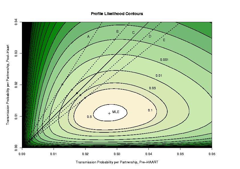
What does this mean? For each pair of transmission probabilities, we have the best possible likelihood we can get (the largest value possible, found by picking the condom protection factor to make it as big as possible). There is a peak labeled with a cross, as you can see. That value represents the maximum likelihood estimate of the transmission probabilities, and notice that the value post-HAART is substantially lower than pre-HAART. We believe this difference to be due to drugs, but this cannot be proven based on these data alone (there is no control group and no possible way to assess the exposure of the partners of the men in the study to the drugs.)

Now, suppose that we assume that the prevalence is the same pre- and post-HAART. Let's now constrain the infectivity to be the same. So with the prevalence the same and the infectivity the same, we have to have the transmission probability be the same before and after HAART. In other words, we have to stay on the 45-degree line on the graph, shown on the figure in solid black. Given that, where is the maximum likelihood estimate? It is at the black dot you see on it; if you stay on that black like, that is the highest elevation you can get to and it represents the best single (lumped) estimate of the transmission probability per partnership. If the height you can get to is not far below the very best (unconstrained) height (at the cross), then the constraint didn't make much difference in a way. If that were to be the case, the data would provide no evidence in favor of a difference. On the other hand, if having to stay on the solid line dramatically lowered the best (greatest) likelihood you could achieve, then that is evidence that you shouldn't have to stay on the solid line: you would reject the hypothesis of constant infectivity (given constant prevalence).

So which is it? We indicated contours that correspond to hypothesis rejection at different alpha levels (by the likelihood ratio chi-square test), and that is what you see on the graph. The solid dot (the maximum likelihood estimate of the transmission probabilities given the hypothesis of no infectivity difference, and constant prevalence) is between the 0.05 contour and the 0.01 contour, so the p-value is between 0.05 and 0.01. So at a level of 0.05, we reject the hypothesis of constant infectivity.

Now, suppose that the prevalence increased post-HAART, since the death rate due to AIDS decreased. Now, if we assume that the infectivity is the same pre- and post-, what happens? We're assuming the prevalence after HAART p₂ is less than the prevalence p₁ pre-HAART. If we pick some infectivity , we can then compute the transmission probability per partnership before and after HAART, respectively, p₁ and p₂. If we do this for a lot of different values of the infectivity and plot the answers, we get a straight line, not at 45-degrees, but sloping upward at a steeper angle (since the prevalence has been assumed to increase but the infectivity is the same, the actual transmission probability per partnership just has to go up.) Given this constraint, what is the best value? You find the highest point on the transect, and see how much lower it is than the overall peak. In our case, the steeper this slope, the lower it is, indicating that if the prevalence actually increased, it is less plausible that the infectivity is the same pre- and post-HAART. In particular, the dotted line A (at to a rejection threshold of 0.001) corresponds to a 57.7% increase in prevalence (but that is really too big to believe). The dotted line B (at rejection threshold of 0.1) corresponds to a 17.2% increase in prevalence.

This goes the other way too. If we assume a prevalence decrease after HAART (maybe people who were negative disproportionately and greatly increased their risk behavior, diluting the positives...but there is no evidence for this mechanism and we looked at our cohort at least). Now, the solutions are constrained on a line with a shallower slope than 45-degrees. The peak along these transects is higher, indicating that there would be less evidence against the hypothesis of constant infectivity. In other words, we would be partially explaining the findings by assuming a decrease in prevalence. Assuming a 9.3% decline in prevalence takes us to the rejection contour of 0.05; if we believe the prevalence decreased by more than 9.3% after HAART was introduced, we can no longer reject the hypothesis of constant infectivity (line D). Finally the 0.10 rejection contour is reached by assuming a 20.4% decline in prevalence.

I'll show how these were constructed in R in the future; this was a somewhat numerically intensive calculation. Crude contour plots can be made with the function contour which I invite you to explore.

Another thing that we did was to compute bootstrap resamples of the data set each wave, and for each resampled data set, used the same algorithm to find the best estimate. One problem, however, arises: in a bootstrap resample, there might be no seroconverters at all, and then the best estimate for the infectivity is zero, right on the boundary. In these cases we had to eliminate this particular beta from the optimization, since we already know what it is.

Another part of the final analysis was to assume a different per-partnership infectivity for a subset of the population, and compute simulated infectivity data based on this assumption. We then fit the simulated data and computed how often we falsely concluded there was a infectivity drop due solely to frailty selection bias (using up the people most likely to be infected, causing the average in the cohort to fall).

In the future we'll add some of this code to this page; more details and complete references can be found in the paper².

In the next lecture, we'll look at a SARS preparedness analysis programmed by Tomas Aragon.

¹Osmond DH, Page K, Wiley J, Garrett K, Sheppard HW, Moss AR, Schrager L, Winkelstein W Jr. HIV infection in homosexual and bisexual men 18 to 29 years of age: the San Francisco Young Men's Health Study. American Journal of Public Health 84:1933-1937, 1994.

² To appear.

³Grant RM, Wiley JA, Winkelstein W. Infectivity of the human immunodeficiency virus: estimates from a prospective study of homosexual men. Journal of Infectious Diseases 156: 189-193, 1987.